Executive Overview
The commercial deployment of Large Language Models (LLMs) has ushered in an era of unprecedented computational demand. Behind the polished application programming interfaces (APIs) of generative AI assistants, enterprise search tools, and autonomous coding agents lies a brutal hardware economic reality: graphics processing units (GPUs)—the indispensable engines of modern artificial intelligence—spend a staggering majority of their operational lives sitting idle.
This paradox of high compute capacity and low resource utilization stems from the idiosyncratic nature of LLM serving. Unlike traditional enterprise workloads or even classical computer vision pipelines, where processing times are uniform and predictable, transformer-based autoregressive models generate output token by token. A single user prompt might result in a concise, five-word confirmation, while another triggers a thousand-word technical essay. Because one request finishes rapidly and another lumbers on for minutes, serving infrastructure faces wild fluctuations in task duration and processing intensity.
Without sophisticated intervention, naive inference pipelines handle these requests sequentially. A prompt arrives, the model processes it through billions of parameters, and the GPU goes dark while waiting for the next transmission—despite possessing the architectural bandwidth to process multiple requests simultaneously at virtually identical operational costs.
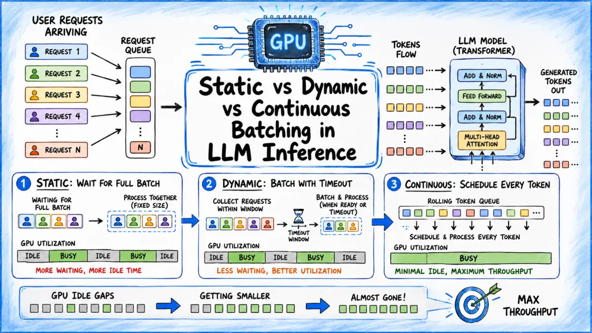
To bridge this economic and computational chasm, infrastructure engineers rely on batching. By grouping multiple independent requests and passing them through the model weights in a single collective operation, systems can transform idle GPU cycles into raw throughput. However, the exact mechanism used to form and manage these batches dictates the difference between an economically viable AI service and a financially ruinous, latency-choked system.
This article explores the evolution of batching mechanics in LLM inference—transitioning from legacy static batching and request-level dynamic batching to modern continuous (or in-flight) batching—and analyzes why these distinctions dictate modern production architecture.
Detailed Chronology: The Architectural Evolution of LLM Batching
To understand why modern LLM serving frameworks operate the way they do, one must trace the evolutionary lineage of inference optimization strategies. As models scaled from millions of parameters to hundreds of billions, the methodologies required to feed them data evolved in lockstep.
Phase 1: The Era of Static Batching (The Bulk-Processing Paradigm)
Static batching represents the most literal, direct interpretation of batch processing borrowed from traditional deep learning and big data pipelines. In a static batching architecture, the inference server is configured with a rigid parameter: a predetermined batch size (e.g., $k = 8$).
[Request 1] ──┐
[Request 2] ──┼──> [ Queue ] ──(Waits until 8 requests accumulate)──> [ Single GPU Forward Pass ]
[Request 3] ──┘
The server establishes an incoming queue. As user prompts arrive, they are held in memory. The system refuses to execute a forward pass until the total count of accumulated requests precisely matches the configured batch size. If seven requests arrive rapidly, but the eighth stalls, all seven preceding requests sit idle in the queue, held hostage by the absence of the final piece of the puzzle.
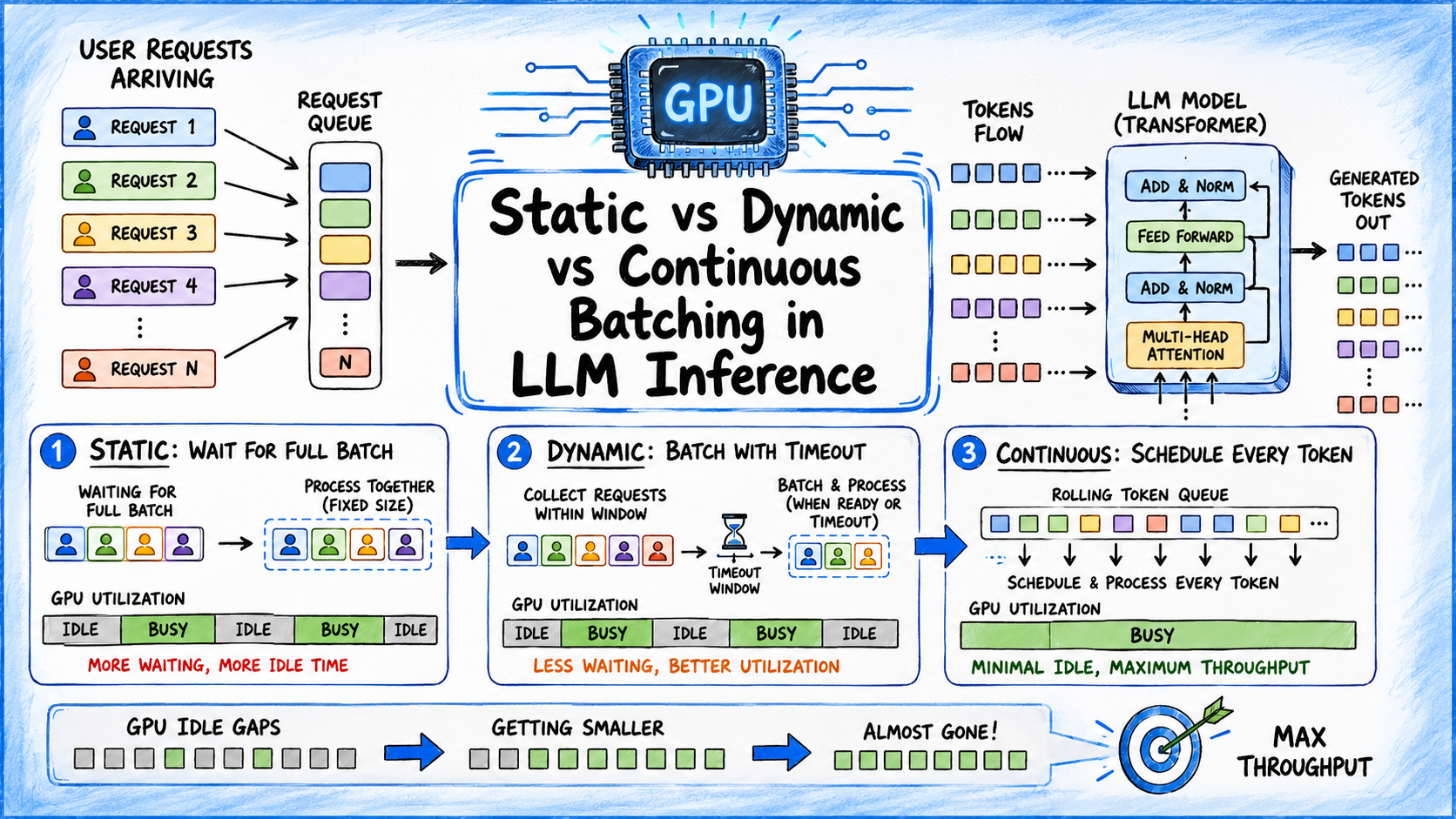
Once the batch threshold is breached, the server bundles the sequences, pads them to uniform lengths, and executes a single forward pass across the shared model weights. The core economic advantage here relies on memory bandwidth amortization. Loading gigabytes of model weights from High Bandwidth Memory (HBM) to the GPU’s compute cores is an expensive operation. Performing this transfer once for eight concurrent requests rather than executing eight independent memory fetches yields a massive efficiency multiplier.
However, static batching was engineered for predictable, non-interactive batch workloads—such as scoring millions of rows in a database or running nightly classification jobs. For live, interactive production traffic characterized by stochastic arrival rates and wildly uneven output lengths, static batching creates unacceptable performance bottlenecks:
- Arbitrary Latency Incurrence: Early arrivals must wait indefinitely for late-arriving peers.
- The "Slowest-Link" Trap: Even within a successfully formed batch, the entire group is bound by the generation duration of the longest request. If seven requests finish in 10 tokens but the eighth requires 500, the GPU must continue running computation passes for the entire batch just to service that single outlier.
Phase 2: The Rise of Dynamic Batching (Introducing Timeouts)
Recognizing the severe limitations of rigid static queues in production web environments, systems architects introduced dynamic batching (frequently pioneered and refined in high-performance serving frameworks like NVIDIA Triton Inference Server).
Dynamic batching retains the core premise of grouping requests to share a single weight-load, but strips away the absolute requirement that a batch must be completely full before execution can commence. Instead, the scheduler introduces two boundary conditions: a maximum batch size and a timeout window (or maximum queue delay).
[Incoming Request] ──> [ Timer Starts ] ──┬──> (Max Batch Size Reached?) ──> [ Execute Batch ]
                                         └──> (Timeout Window Expires?)   ──> [ Execute Partial Batch ]
Under this model, the moment the first request of a new batch arrives, a low-overhead timer is triggered. The server monitors the incoming queue:
- If enough subsequent requests arrive to hit the maximum batch size before the timer expires, the batch is dispatched immediately (identical to static batching).
- If the timer expires before the batch fills, the server abandons the quest for completeness and fires a partial batch containing whatever requests have accumulated thus far.
This innovation successfully bounds the worst-case queuing latency, making live, real-time endpoints viable. High-traffic periods naturally fill maximum batch sizes, maximizing throughput, while low-traffic lulls trigger timeouts, ensuring that users do not experience infinite wait times.
Despite this advancement, dynamic batching leaves the second fundamental flaw of batch processing untouched: intra-batch synchronization. Once a dynamically formed batch begins its execution loop, all member requests are bound together. The system still waits for the completion of the longest sequence in the batch before freeing up compute resources, cementing the penalty of uneven token generation lengths.
Phase 3: The Paradigm Shift to Continuous Batching (In-Flight Scheduling)
The structural mismatch between autoregressive LLM generation and traditional batching was finally resolved with the introduction of continuous batching (also referred to in various ecosystems as in-flight batching or iteration-level scheduling).
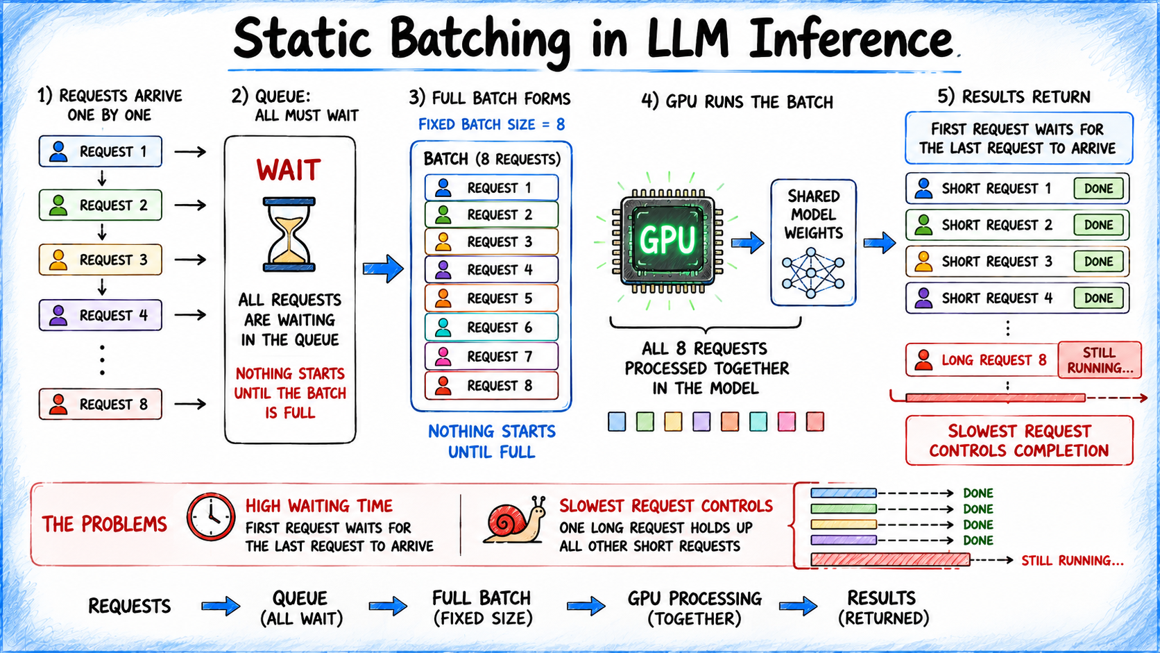
Pioneered academically and rapidly adopted by modern high-performance frameworks such as vLLM, TensorRT-LLM, and Text Generation Inference (TGI), continuous batching fundamentally reimagines the scheduling unit. It abandons the "request" or "entire batch" as the fundamental unit of scheduling, replacing it with the individual decoding iteration (step).
Iteration 1: [Seq A (Token)] [Seq B (Token)] [Seq C (Token)]
               (Seq C finishes with <EOS>)
Iteration 2: [Seq A (Token)] [Seq B (Token)] [New Seq D (Token)]
In a continuous batching runtime, the inference engine maintains a rolling pool of active sequences. At every single decoding step (forward pass), the server processes one token for every active sequence currently in the pipeline.
The lifecycle mechanics operate as follows:
- Dynamic Insertion: If a new request arrives while the GPU is actively processing generation steps for other users, it does not wait in a static queue or timeout window. Instead, it is injected directly into the active batch on the very next decoding iteration, provided there is available memory capacity.
- Immediate Eviction: The moment a specific sequence emits an
<EOS>(End-of-Sequence) token or reaches its maximum token limit, it is instantly excised from the active batch. - Slot Backfilling: The computational slot vacated by the completed request does not sit empty until the rest of the batch finishes. On the immediate next iteration, a waiting request from the queue steps into that exact slot.
This rolling, asynchronous model means that the composition of the GPU’s active batch mutates on nearly every single clock cycle. The GPU is kept in a state of near-continuous saturation, entirely liberated from the tyranny of waiting for outliers to conclude.
Supporting Context & Metrics: Performance and Trade-Offs
To fully appreciate why continuous batching has become the undisputed gold standard for production LLM serving, one must examine the empirical performance trade-offs governing these three architectures.
Comparative Analytical Metrics
| Strategy | Scheduling Unit | GPU Idle Time | Latency Behavior | Best Production Fit |
|---|---|---|---|---|
| Static Batching | Whole batch | High between batches | High, strictly bound by the slowest request in the batch. | Offline batch jobs, asynchronous dataset scoring, non-interactive pipelines. |
| Dynamic Batching | Whole batch with timeout | Moderate | Bounded by max batch size or timeout window; vulnerable to intra-batch padding overheads. | Fixed-length generation tasks (e.g., specific embedding models, image generation workflows). |
| Continuous Batching | Individual decode step | Minimal / Negligible | Variable per request, but optimized for maximum global throughput and minimal tail latency ($P_99$). | Production autoregressive LLM serving (chatbots, agents, API endpoints). |
Throughput vs. Time-to-First-Token (TTFT) Dynamics
While continuous batching dominates under heavy, concurrent enterprise workloads, performance engineers must account for nuanced operational trade-offs under varying traffic conditions:
- Under Heavy Concurrency: Continuous batching yields exponential throughput improvements over static and dynamic approaches. By eliminating internal fragmentation and ensuring that GPU compute cores are never starved waiting for batch completion, hardware utilization regularly exceeds 80–90% in optimal vLLM configurations.
- Under Light / Sparse Workloads: Ironically, under extremely light traffic where request contention is near zero, request-level dynamic batching can occasionally exhibit a slight edge in Time-to-First-Token (TTFT) due to lighter scheduler overhead. However, production environments rarely maintain static, predictable low-load states; traffic spikes unpredictably, rendering systems optimized exclusively for low-load scenarios dangerously brittle.
Official Industry Perspectives & Architectural Standards
The industry-wide migration toward continuous batching is reflected in the official documentation and release notes of foundational AI infrastructure projects.
NVIDIA’s TensorRT-LLM engineering team highlights the necessity of In-Flight Batching (their proprietary terminology for continuous batching) in technical whitepapers:

"Traditional static and dynamic batchers treat the entire generation lifespan of a prompt as an indivisible block. For autoregressive models, where sequence lengths vary dynamically by orders of magnitude, this introduces catastrophic internal fragmentation. In-flight batching deconstructs the generation loop, allowing the inference engine to schedule computation at the granularity of individual transformer blocks and decode steps, thereby reclaiming up to 10× throughput gains in high-concurrency environments."
Similarly, the maintainers of vLLM emphasize that continuous batching, when paired with advanced memory management techniques like PagedAttention, fundamentally alters the economics of hosting open-weights models (such as Llama 3 or Mistral). By virtualizing KV-cache memory and matching it with iteration-level scheduling, platforms can eliminate memory waste caused by pre-allocating contiguous buffers for maximum possible sequence lengths, allowing server operators to pack significantly more concurrent user sessions onto a single NVIDIA H100 or A100 GPU.
Future Outlook: The Next Frontier in Inference Optimization
As large language models evolve toward multimodal capabilities (processing simultaneous interleaved streams of text, audio, video, and high-resolution imagery) and reasoning architectures (such as test-time compute scaling and multi-step chain-of-thought generation), the demands on batching schedulers will intensify.
Future research directions are focusing on several key areas:
- Heterogeneous Batching: Dynamically grouping requests that utilize different LoRA (Low-Rank Adaptation) adapters or quantization precisions within the same continuous batching loop without sacrificing hardware execution efficiency.
- Predictive Schedulers: Integrating lightweight machine learning models directly into the inference router to predict token generation lengths a priori, allowing continuous batching schedulers to pre-emptively slot requests with mathematical precision rather than reactive heuristics.
- Disaggregated Serving: Separating the prefill (prompt processing) phase from the decode (token generation) phase across specialized physical GPU pools. Because prefill operations are compute-bound and decode operations are memory-bandwidth bound, disaggregated architectures require entirely novel, cross-node continuous batching paradigms to route intermediate states seamlessly.
For production engineers, platform architects, and enterprise decision-makers, understanding these batching tiers is no longer an academic exercise. It is the core determinant of whether an AI application can scale economically or collapse under the weight of its own infrastructure costs.